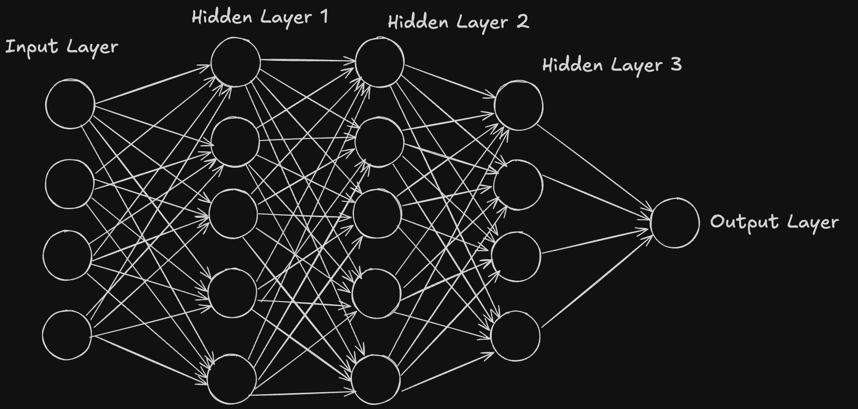
Building a Neural Network from Scratch

We’ll build a very basic neural network using Python, without using any deep learning libraries. We'll also walk through the basic ideas of how neural networks work and create a simple neural network that learns to solve a small problem (XOR).

What is a Neural Network?

A neural network is a type of machine learning model that is inspired by how the human brain works. It is made up of layers of neurons (or nodes), each connected to others by weights. These connections help the network learn patterns in the data.

A basic neural network has:

Input Layer: Where the data comes in.
Hidden Layer: Where the data is processed.
Output Layer: Where the result or prediction comes out.

Neural Network

How It Works

Each neuron in a layer gets input, multiplies it by a weight, and adds a bias.
The result is passed through an activation function (like Sigmoid) to get the output.
The neural network adjusts the weights and biases to make the output closer to the desired result (this process is called training).

Step 1: Initialize Our Network

First, we need to create a neural network with:

Input Layer: 2 nodes (because we'll use two input features)
Hidden Layer: 4 nodes (this can be adjusted)
Output Layer: 1 node (since we’re solving a binary problem like XOR)

We'll also initialize weights (how strongly each input influences the output) and biases (to shift the activation function).

import numpy as np
 
class NeuralNetwork:
    def __init__(self, input_size, hidden_size, output_size):
        # Randomly initialize weights and biases
        self.W1 = np.random.randn(input_size, hidden_size)  # Weights for input to hidden
        self.b1 = np.zeros((1, hidden_size))  # Bias for hidden layer
        
        self.W2 = np.random.randn(hidden_size, output_size)  # Weights for hidden to output
        self.b2 = np.zeros((1, output_size))  # Bias for output layer

Step 2: Forward Propagation

Forward propagation means passing the data through the network to get an output.

Multiply inputs by weights, add biases, and pass through an activation function (we'll use Sigmoid here).

def sigmoid(self, z):
    return 1 / (1 + np.exp(-z))  # Sigmoid activation function
 
def forward(self, X):
    # Calculate the output for the hidden layer
    self.z1 = np.dot(X, self.W1) + self.b1  # Weighted sum of inputs
    self.a1 = self.sigmoid(self.z1)  # Activation
 
    # Calculate the output for the final layer
    self.z2 = np.dot(self.a1, self.W2) + self.b2
    self.a2 = self.sigmoid(self.z2)  # Final output (prediction)
    return self.a2

In forward propagation:

We calculate the weighted sum of inputs for the hidden layer.
Pass this through a Sigmoid function to get the activation (output) of the hidden layer.
Repeat for the output layer to get the final prediction.

Step 3: Backpropagation

Backpropagation is how the neural network learns. It adjusts the weights to make the predictions more accurate.

Here, we use Mean Squared Error (MSE) to measure the difference between the predicted output and the actual result. Then, we update the weights using the gradients (how much the weights affect the output).

def sigmoid_derivative(self, z):
    return self.sigmoid(z) * (1 - self.sigmoid(z))  # Derivative of Sigmoid
 
def backward(self, X, y):
    m = X.shape[0]  # Number of training examples
    
    # Calculate error at the output layer
    dZ2 = self.a2 - y
    dW2 = np.dot(self.a1.T, dZ2) / m
    db2 = np.sum(dZ2, axis=0, keepdims=True) / m
    
    # Calculate error at the hidden layer
    dZ1 = np.dot(dZ2, self.W2.T) * self.sigmoid_derivative(self.z1)
    dW1 = np.dot(X.T, dZ1) / m
    db1 = np.sum(dZ1, axis=0, keepdims=True) / m
    
    # Update weights and biases
    self.W1 -= 0.1 * dW1  # Learning rate is 0.1
    self.b1 -= 0.1 * db1
    self.W2 -= 0.1 * dW2
    self.b2 -= 0.1 * db2

What happens in Backpropagation?

We calculate how much the output error is influenced by each weight.
We adjust the weights and biases in the direction that reduces the error.

Step 4: Training the Network

Now, we train the network! We will run forward propagation and backpropagation for many iterations (epochs) to improve the model's predictions.

def train(self, X, y, epochs):
    for epoch in range(epochs):
        output = self.forward(X)  # Get the predicted output
        self.backward(X, y)  # Update weights using backpropagation
        
        # Optionally print loss every 100 epochs
        if epoch % 100 == 0:
            loss = np.mean((output - y) ** 2)  # Mean Squared Error loss
            print(f"Epoch {epoch} - Loss: {loss}")

Training Steps:

Forward pass: Get predictions.
Backward pass: Adjust weights and biases.
Repeat for many epochs (iterations) to make the model better.

Putting It All Together

Let’s test our neural network with a simple problem, XOR, where the output is 1 if the inputs are different and 0 if they are the same.

XOR Problem Example:

# XOR input and output
X = np.array([[0, 0], [0, 1], [1, 0], [1, 1]])  # Input
y = np.array([[0], [1], [1], [0]])  # Expected output
 
# Create the neural network
nn = NeuralNetwork(input_size=2, hidden_size=4, output_size=1)
 
# Train the neural network
nn.train(X, y, epochs=10000)

In this code:

X is the input (two features).
y is the output (XOR values).

After training, the network will learn how to predict XOR outputs based on the inputs.

Conclusion

You’ve just built a simple neural network from scratch! In this tutorial, we:

Created a neural network with one hidden layer.
Implemented forward propagation to make predictions.
Used backpropagation to adjust weights and minimize the error.
Trained the network on the XOR problem.

This is just a starting point. Neural networks can become much more complex, but understanding this basic structure is the key to building more advanced models!

References:

Happy learning and coding!